Logistic Equation version 2: Solve a first-order ODE

This is part 2 in a series introducing the ode45 solver for integrating the logistic equation, a first-order ODE:

In this version, we demonstrate how to set the relative and absolute tolerances and compare the numerical solution to the analytic solution that is given by:

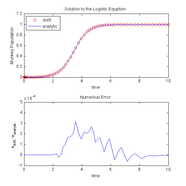
The plot below shows how the numerical error changes with time. Notice that the error is large where the value of x undergoes rapid changes. In this example, the relative tolerance (defined below) is set to 1e-3. The maximum value of the actual error is consistent with this value, although that is not always guaranteed (your mileage may vary...).

Download logisticV2.m

% logisticV2.m
%
% Numerically integrate a 1D ODE (the Logistic Equation) using the
% Runge-Kutta 45 solver and and compare the result to the analytic solution
%
function logisticV2
a = 2;          % free parameter

tBegin = 0;     % time begin
tEnd = 10;      % time end

x0 = 0.001;     % initial position

% Use the Runge-Kutta 45 solver to solve the ODE
% Set relative and absolute tolerances
options = odeset('RelTol', 1e-3, 'AbsTol', 1e-6);
[t,x] = ode45(@derivatives, [tBegin tEnd], x0, options);

% Analytic Solution
x2 = x0 ./ ((1-x0) * exp(-a*t) + x0);


%%%%%  top plot:  solutions
subplot(2,1,1)      % top plot
plot(t,x,'ro');     % plot ode45 solution as red circles
hold on             % superimpose next plot on previous
plot(t,x2,'b-');    % plot analytic solution as blue line
ylim([0 1.2]);      % set y plot limits

title('Solution to the Logistic Equation');             % title
xlabel('time');                                         % label x axis
ylabel('Monkey Population');                            % label y axis
legend('rk45', 'analytic', 'Location', 'Northwest')     % legend top left


%%%%%  lower plot:  error
subplot(2,1,2)                      % lower plot
plot(t,x-x2,'b-')                   % plot error as blue line
title('Numerical Error');           % Title
xlabel('time');                     % label x axis
ylabel('x_{rk45}-x_{analytic}');    % label y axis


% print to pdf
set(gcf, 'PaperSize', [6 6]);
set(gcf, 'PaperPosition', [0 0 6 6]);
print ('-dpdf','logisticV2.pdf');
print ('-dpng','logisticV2.png','-r100');


    %%%%%  Function: derivatives
    % returns the derivative dx/dt for the logistic equation
    % uses the parameter a from main program, but changeth it not
    function dxdt = derivatives(t,x)
        dxdt = a * x * (1 - x);
    end

end

Monkey Commentary

In version 2 of the code, we set the relative and absolute tolerances through the options:

options = odeset('RelTol', 1e-3, 'AbsTol', 1e-6);
[t,x] = ode45(@derivatives, [tBegin tEnd], x0, options); 

It is important to understand that these tolerances are not with respect to the actual solution (we usually do not know the actual solution). Rather, the ode45 routine calculates the values using both 4th order and (presumably more accurate) 5th order Runge-Kutta methods. The tolerance specifies how much these two estimates of the true solution can differ. The ode45 routine keeps reducing the time step until the difference between the 4th and 5th order solutions fall within the specified tolerance range. Thus, reducing the tolerances usually produces a more accurate solution (but not always).

Generally speaking, the absolute tolerance controls the time step when the solution is close to zero, and the relative tolerance controls it when the solution is far from zero.

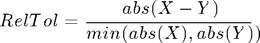
RelTol is a measure of the error relative to the size of each solution component. Roughly, it controls the number of correct digits in all solution components, except those smaller than the AbsTol threshhold. The default value, 1e-3, corresponds to 0.1% accuracy. The relative tolerance between two numbers X and Y is defined as

Since this expression blows up when X or Y approaches zero, a separate absolute tolerance AbsTol is invoked near zero. AbsTol is a threshold below which the value of the ith solution component is unimportant. The absolute error tolerances determine the accuracy when the solution approaches zero. The default value is 1e-6.

We recommend monkeying around with the tolerance values to see how they affect the resulting errors in this example.

---

Home   |   Plot Thumbnails   |   Prev: Plotting   |   Next: Plotting