Solve a 2nd Order ODE: Damped, Driven Simple Harmonic Oscillator

This example builds on the first-order codes to show how to handle a second-order equation. We use the damped, driven simple harmonic oscillator as an example:

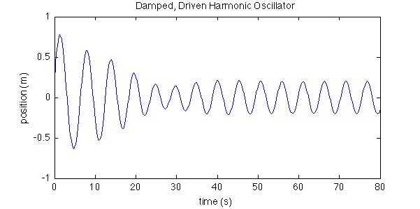
In a second order system, we must specify two initial conditions. In the plot shown below we choose

We assume MKS units, but this is unimportant for our discussion. The system is resonant when the driving frequency matches the natural frequency. We choose our parameters near resonance:

The following figure shows the result. The dynamics show initial transient behavior which gives way to resonant oscillations.

Download resonance.m

% resonance.m
% Numerically integrate second-order ODE: Damped, driven harmonic oscillator

function resonance

omega = 1;      % resonant frequency = sqrt(k/m)
b = 0.2;        % drag coeficient per unit mass
A = 0.1;        % driving amplitude per unit mass
omega0 = 1.2;   % driving frequency

tBegin = 0;     % time begin
tEnd = 80;      % time end

x0 = 0.2;       % initial position
v0 = 0.8;       % initial velocitie

a = omega^2;    % calculate a coeficient from resonant frequency

% Use Runge-Kutta 45 integrator to solve the ODE
[t,w] = ode45(@derivatives, [tBegin tEnd], [x0 v0]);
x = w(:,1);     % extract positions from first column of w matrix
v = w(:,2);     % extract velocities from second column of w matrix

plot(t,x);

title('Damped, Driven Harmonic Oscillator');
ylabel('position (m)');
xlabel('time (s)');


    % Function defining derivatives dx/dt and dv/dt
    % uses the parameters a, b, A, omega0 in main program but changeth them not
    function derivs = derivatives(tf,wf)
        xf = wf(1);            % wf(1) stores x
        vf = wf(2);            % wf(2) stores v
        dxdt = vf;                                     % set dx/dt = velocity
        dvdt = -a * xf - b * vf + A * sin(omega0*tf);  % set dv/dt = acceleration
        derivs = [dxdt; dvdt];  % return the derivatives
    end

end

Monkey Commentary

We compare the differences between the first order code (logisticV1.m) this code. Because the derivatives routine must reference both position and velocity, we 'package' these variables into a single array we call wf. Inside the derivatives function, we then 'unpack' the variables of interest (position xf and velocity xf in this case):

       xf = wf(1);            % wf(1) stores x
       vf = wf(2);            % wf(2) stores v  

Notice that because variables x and v are used in the main program, we choose different variable names in the function: xf and vf. Otherwise, the main program variables x and v will be overwritten and complete monkey chaos will ensue. We stick an 'f' on each of the variables to indicate they reside in our function...

Next, we calculate the derivatives. Because we are solving a second order system, we need to return two derivatives:

       dxdt = vf;                                         % set dx/dt = velocity
       dvdt = -a * xf - b * vf + A * sin(omega0*tf);      % set dv/dt = acceleration

In a second-order system the first derivative dxdt is just be set to the velocity variable. The velocity derivative dvdt contains the interesting information defining the acceleration.

We package up our derivatives and stuff them in a new array we call derivs:

derivs = [dxdt; dvdt];  % return the derivatives 

This variable derivs must be the same variable name used in defining the function:

function derivs = derivatives(tf,w)

Now back to the main program. The ode45 function returns our packaged dependent variables and the independent variable, which we call w and t. As before, we need to unpack our variable w to retreive the position x and velocity v data:

[t,w] = ode45(@derivatives, [tBegin tEnd], [x0 v0]);
x = w(:,1);     % extract positions from first column of w matrix
v = w(:,2);     % extract velocities from second column of w matrix

That's it! The variables x and v contain the solutions we desired. We can now plot them or use them in in other calculations.

---

Home   |   Plot Thumbnails   |   Prev: Plotting   |   Next: Plotting