Addendum to Kepler's Equation: Error Analysis

In the code KeplerEquation.m we tracked an orbiting body through one period of an elliptical orbit. It used a series expansion involving Bessel functions to solve Kepler's equation. In the code keplerEquationError.m we evaluate the accuracy of this method when a finite number of terms are included in the series expansion.

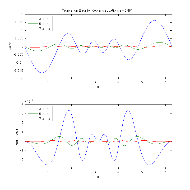
The following plot shows the error as a function of the angle theta for three different cases: when the infinite series is truncated at the 3rd, 5th and 7th terms for an ellipse with an eccentricity of 0.4. With only 5 terms, the error as dropped to less than 0.1%.

Download KeplerEquationError.m

% KeplerEquationError.m
%
% This code estimates errors in the orbital positions calculated using
% the Bessel function expansion of Kepler's equation (see KeplerEquation.m)
% It plots the errors as a function of the angle theta for three different
% cases:  when the infinite series is truncated at the 3rd, 5th and 7th terms
%
% MATLAB-Monkey.com  10/1/2013


%%%%%%%%%%
%%%%%%%%%%  Parameters & Initialization
%%%%%%%%%%

clear           % clear variables
clc             % clear command window

e = 0.4;        % eccentricity
a = 1;          % semi-major axis
N = 100;        % number of points defining orbit

nTerms = [3 5 7]; % number of terms kept in eccentric anomaly series

M = linspace(0,2*pi,N);   % mean anomaly parameterizes time
                          % M varies from 0 to 2*pi over one orbit

alpha = zeros(1,N);       % preallocate space for eccentric anomaly array



%%%%%%%%%%
%%%%%%%%%%  Calculations & Plotting
%%%%%%%%%%


%%%%%%%%%%  Estimate the "true" solution by using 30 terms in the infinite series

% Calculate eccentric anomaly at each point in orbit
for j = 1:N
    % initialize eccentric anomaly to mean anomaly
    alpha(j) = M(j);

    % include first nTerms in infinite series
    for n = 1:30
        alpha(j) = alpha(j) + 2 / n * besselj(n,n*e) .* sin(n*M(j));
    end
end

% calcualte polar coordiantes (theta, r) from eccentric anomaly
theta30 = 2 * atan(sqrt((1+e)/(1-e)) * tan(alpha/2));
theta30(theta30<0) = theta30(theta30<0) + 2*pi;
r30 = a * (1-e^2) ./ (1 + e*cos(theta30));




%%%%%%%%%%  Orbit calculation with restricted number of terms

% loop through elements of matrix nTerms
for k = 1:length(nTerms)

    % Calculate eccentric anomaly at each point in orbit
    for j = 1:N
        % initialize eccentric anomaly to mean anomaly
        alpha(j) = M(j);

        % include first nTerms in infinite series
        for n = 1:nTerms(k)
            alpha(j) = alpha(j) + 2 / n * besselj(n,n*e) .* sin(n*M(j));
        end
    end

    % calcualte polar coordiantes (theta, r) from eccentric anomaly
    theta = 2 * atan(sqrt((1+e)/(1-e)) * tan(alpha/2));
    theta(theta<0) = theta(theta<0) + 2*pi;
    r = a * (1-e^2) ./ (1 + e*cos(theta));

    % find error
    thetaError = theta - theta30;
    rError = r - r30;

    % plot errors as a function of theta
    subplot(2,1,1)
    plot(theta30,thetaError)
    hold all

    subplot(2,1,2)
    plot(theta30,rError)
    hold all

    % create entry for legend indicating max number of terms
    legendText{k} = sprintf('%i terms',nTerms(k));
end

% label plots and create legend
subplot(2,1,1)
title(sprintf('Truncation Error for Kepler''s equation (e = %.2f)',e));
xlim([0 2*pi]);
xlabel('\theta');
ylabel('\theta error');
legend(legendText,'Location','Northwest')

subplot(2,1,2)
xlim([0 2*pi]);
xlabel('\theta');
ylabel('radial error');
legend(legendText,'Location','Northwest')


% Save plot as pdf
set(gcf, 'PaperPosition', [0 2 8 8]);
print ('-dpdf','kepler.pdf');
print ('-dpng','kepler.png','-r300');

---

Home   |   Plot Thumbnails   |   Prev: Plotting   |   Next: Plotting