
CRTBP Pseudo-Potential and Lagrange Points
1. Pseudo-Potential
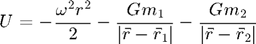
When the motion of the test particle is confined to the plane containing the massive bodies, the acceleration in the rotating reference frame may be written in the form:

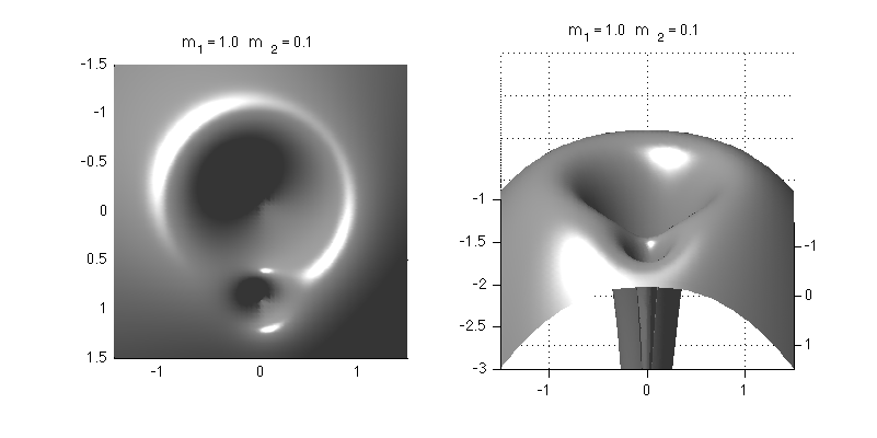
The following figure shows the potential represented as a surface plot for a mass ratio of m2/m1 = 0.1:
Downloads:
- crtbpPotentialSurface.m - Plots the surface of the pseudo-potential for the circular, restricted three-body. Requires crtbpPotential.m to run.
Dependent files:
- crtbpPotential.m - returns the pseudo-potential for the circular, restricted three-body
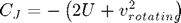
2. Jacobi Integral and Zero-Velocity Curves
While neither energy nor angular momentum are conserved in the rotating reference frame of the CRTBP, there is a quantity that is a constant of the motion. This quantity is called the Jacobi integral:
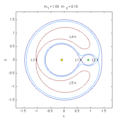
The following figure shows zero velocity curves for different Jacobi integrals. The zero-velocity curves bound the shaded 'forbidden' regions where a particle with the specified Jacobi integral can not venture. For example, if a particle with CJ = 4 is initially in orbit around the green planet, it will be stuck there forever (unless it is given a velocity boost by some means). However, the zero-velocity curve for CJ = 3.92 encompasses both m1 and m2. Therefore a particle with this value of CJ can transition back and forth between orbits around each object.
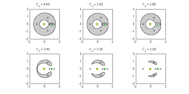
This plot also show the positions of the five Lagrange points (see next section).
Downloads:
- crtbpZeroVel.m - Plots zero-velocity curves for difference values of the Jacobi integral. Also marks the positions of the Lagrange points with "+" symbols. Requires crtbpPotential.m and lagrangePoints.m to run.
Dependent files:
- crtbpPotential.m - returns the pseudo-potential for the circular, restricted three-body
- lagrangePoints.m - returns a matrix containing the (x,y,z) coordinates of the five Lagrange points for given values of m1 and m2. This routine assumes that G = 1 and the distance between the primary objects in 1.
3. Lagrange Points
Lagrange points (a.k.a. libration points) are equilibrium points in the rotating frame. They correspond to places where the pseudo-potential is locally flat. Lagrange showed that there are five such points for any mass ratio m2/m1. Two Lagrange points, L4 and L5, form an equilateral triangle with the two primary masses, one above the masses and the other below. The remaining three Lagrange points L1, L2, L3 lie along the line containing m1 and m2. The positions of the colinear points require solving the roots of a set of fifth order polynomials. The MATLAB program lagrangePoints.m determines the solution numerically for given masses m1 and m2.
Downloads:
- LagrangePlot.m - Plots the Lagrange points and the zero-velocity curves that pass through them for a given m1 and m2.
Dependent files:
- crtbpPotential.m - returns the pseudo-potential for the circular, restricted three-body
- lagrangePoints.m - returns a matrix containing the (x,y,z) coordinates of the five Lagrange points for given values of m1 and m2. This routine assumes that G = 1 and the distance between the primary objects in 1.