Solve a 2D, Second-Order ODE: 2D Spring Motion

Continuing our study of ODEs, this example is a two-dimensional, second-order ODE. Two springs with spring constants k1 and k2 are attached to a mass: the first along the x axis, the second along the y axis. The amplitude of the oscillations is assumed small so we can treat the x and y motions as independent. The natural frequencies in the x and y directions are omega1 and omega2, respectively.

The equations of motion are:

Because these two equations are completely decoupled, we could solve them independently. However, we choose to solve them simultaneously to to illustrate how to set up a 2D system in MATLAB.

In a 2D, second-order system, we must specify four initial conditions. In the plot shown below we choose

This system has only two free parameters, the natural frequencies in the x and y directions:

Because the x- and y-components of the accelerations are independent, the solutions to this set of equations are just Lissajous patterns. In this figure, the plot markers are spaced evenly in time rather than being tied to the adaptive time steps. Thus, markers that are close together indicate that the mass is moving more slowly, and markers that are spread apart more show where the mass is moving more quickly. We discuss how to do this in the commentary at the bottom of the page. The red dot marks the starting location.

Download twoSprings.m

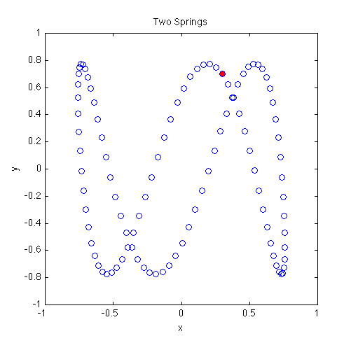
% twoSprings.m
%
% Numerically integrate a two-dimensional, second-order ODE
% Two springs are attached to a mass: one along the x axis, the other along
% the y axis. The amplitude of the oscillations is assumed small so we can
% treat the x and y motions as independent.
%
% We define the natural frequencies in the x and y directions as omega1 and
% omega2, respectively.
%
% The equations of motion are:
% d^2x/dt^2 = -(omega1)^2 * x
% d^2y/dt^2 = -(omega2)^2 * y
%
% MATLAB-Monkey.com   9/29/2013

function twoSprings

omega1 = 1;      % resonant frequency in x direction
omega2 = 3;      % resonant frequency in y direction

tBegin = 0;      % time begin
tEnd = 2*pi;     % time end
nPoints = 100;   % number of times to sample ODE solution

% Define equally-spaced times to sample the ODE solution
times = linspace(tBegin,tEnd,nPoints);

x0 = 0.3;       % initial x position
y0 = 0.7;       % initial y position
vx0 = 0.7;      % initial x component of velocity
vy0 = -1;       % initial y component of velocity


% Use Runge-Kutta 45 integrator to solve the ODE
[t,w] = ode45(@derivatives, times, [x0 y0 vx0 vy0]);

x = w(:,1);      % extract x positions from first column of w matrix
y = w(:,2);      % extract y positions from second column of w matrix
vx = w(:,3);     % extract vx from third column of w matrix
vy = w(:,4);     % extract vy from forth column of w matrix

plot(x,y,'bo');
hold on
plot(x(1),y(1),'bo','MarkerFaceColor','r');  % Mark the initial position with a red dot

axis equal
xlim([-1 1]);
ylim([-1 1]);

title('Two Springs');
ylabel('y');
xlabel('x');


    % Function defining derivatives dx/dt and dv/dt
    % uses the global parameters omega1 & omega2 but changeth them not
    function derivs = derivatives(tf,wf)
        xf = wf(1);            % w(1) stores x
        yf = wf(2);            % w(1) stores y
        vxf = wf(3);           % w(2) stores vx
        vyf = wf(4);           % w(2) stores vy

        dxdt = vxf;            % set dx/dt = x component of velocity
        dydt = vyf;            % set dy/dt = y component of velocity

        dvxdt = -omega1^2 * xf;  % set dv/dt = acceleration
        dvydt = -omega2^2 * yf;  % set dv/dt = acceleration
        derivs = [dxdt; dydt; dvxdt; dvydt];  % return the derivatives
    end

end

Monkey Commentary

Once again, we compare the differences between this code and the previous code (resonance.m). The derivatives routine is structured very similarly. We now have four variables to track (x, y, vx, vy), but we 'pack' and 'unpack' them in the w array just like we did before.

Another difference between this code and the previous code is how the times returned from the ode45 routine are calculated. Previously, we passed a matrix containing the begin time and end time as the second parameter to the ode45 routine:

previous code:
[t,w] = ode45(@derivatives, [tBegin tEnd], [x0 y0 vx0 vy0]);   

The returned t array contained the times of every time step used in solving the ODE. Thus, when the solver reduced the time step to increase accuracy, the times that were returned in the t array were also closer together. In the present code, we pass an array containing 100 values, ranging from tBegin to tEnd. When this array contains more than two values (as it does in the present example), the ode45 routine will only return the component values that correspond to the times contained in the times array, i.e. they are independent of the actual time steps used in solving the ODE. This is useful because we would like the relative spacing of the data points to reflect the velocity of the particle rather than the time step used by the integrator.

times = linspace(tBegin,tEnd,nPoints);
...
[t,w] = ode45(@derivatives, times, [x0 y0 vx0 vy0]);   

---

Home   |   Plot Thumbnails   |   Prev: Resonance   |   Next: Plotting